Evernote Export

Matlab基础

Matlab基础

MATLAB的基本运算

MATLAB的数据类型

变量

Matlab的变量无需事先声明，也不需指定类型。
命名规则

变量名区分大小写。
变量名必须以字母开头，可包含字母，数字和下划线。
变量名长度不超过63个。

常用常量

常量	说明
eps	浮点运算的相对精度
i，j	虚数单位
Inf	无穷大
NaN	不定值（0/0）

变量类型（比较重要的）

数值型	说明
double	双精度浮点型默认类型
int	整型
char	字符型
syms a b c	多个符号变量a，b，c

注意字符型和符号变量的区别

元胞数组cell

元胞数组由元胞组成
元宝可以存放任意类型，大小的数组
元胞的操作：

%定义
A={[1,2,3],ones(3),'matlab'}
%调用
>>A{1,1}

ans=
        1   2   3

A=cell(1,3);
A{1,1}=[1,2,3];
A{1,2}=ones(3);
A{1,3}='matlab';

以上两种方式等价

注意元胞和矩阵的区别, A{1,2}≠A[1,2]

结构体struct

结构体的定义：以下两种方式等价

%直接定义
A.b1=1;
A.b2=ones(2);
A.b3='matlab';

%通过struct函数生成
A=struct('b1',1,'b2',one(2),'b3','matlab');

调用

>>A.b1

ans=
            1

函数句柄

间接调用函数-

矩阵运算

矩阵生成

函数	说明	函数	说明
zeros	全0矩阵	diag	对角阵
ones	全1矩阵	eye	单位矩阵
rand	均匀分布随机矩阵
调用方式	fun为任意上述函数	---	---
fun(n)	生成n阶上述方阵	fun(n)	---
fun(m,n)	生成m* n阶上述矩阵	/	/

矩阵元素调用

输入	说明
A(m,n)	第m行第n列
A(m ; :)	第m行
A(: ; n)	第n列

向量的生成

x=x0 : Δx : xn
x=linspace(x1 , xn , n)

矩阵的基本操作

函数名	说明
det	求行列式
inv	求逆
eig	求特征值和特征向量
rank	求秩
trace	求迹
norm	求范数
poly	求特征方程的系数

输出特征值

>> A=[1,2,3;4,5,6;7,8,9];
>> a=eig(A)

特征值分解

>>[V,D]=eig(A)


V =

   -0.2320   -0.7858    0.4082
   -0.5253   -0.0868   -0.8165
   -0.8187    0.6123    0.4082


D =

   16.1168         0         0
         0   -1.1168         0
         0         0   -0.0000

其中V−1AV=D
D=diag{ λ1 , λ2 , λ3}
3. 特征值分解

>>[V,D,W] = eig(A)


V =

   -0.2320   -0.7858    0.4082
   -0.5253   -0.0868   -0.8165
   -0.8187    0.6123    0.4082


D =

   16.1168         0         0
         0   -1.1168         0
         0         0   -0.0000


W =

   -0.4645   -0.8829    0.4082
   -0.5708   -0.2395   -0.8165
   -0.6770    0.4039    0.4082

V,D同上
WTA(W−1)T=D
即
W−1ATW=D

关系运算

函数	说明
any	任意元素不为0时为真
all	所有元素不为0时为真
find	寻找非0元素坐标

复数及其运算

函数	说明
abs	求模
real	求实部
imag	求虚部
conj	求共轭
angle	求幅角
isreal	判断是否为实数

MATLAB图形可视化

二维图形

基本函数

函数	说明
plot	散点图
plotyy	双y轴散点图
subplot	创建子图
gplot	拓扑图

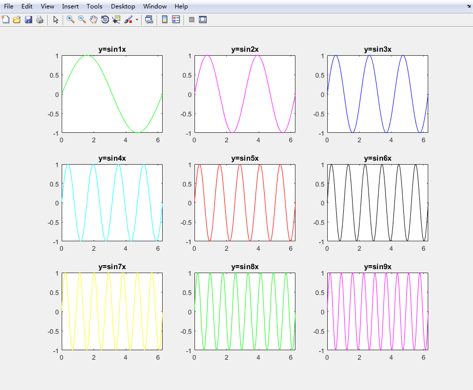
subplot

clc,clear,close all
x=linspace(0,2*pi,200);
b=['g','m','b','c','r','k','y','g','m'];
for m=1:9
    subplot(3,3,m);
    plot(x,sin(m*x),b(m));
    title(['y=sin',num2str(m),'x']);
    axis([0,2*pi,-1,1]);
end

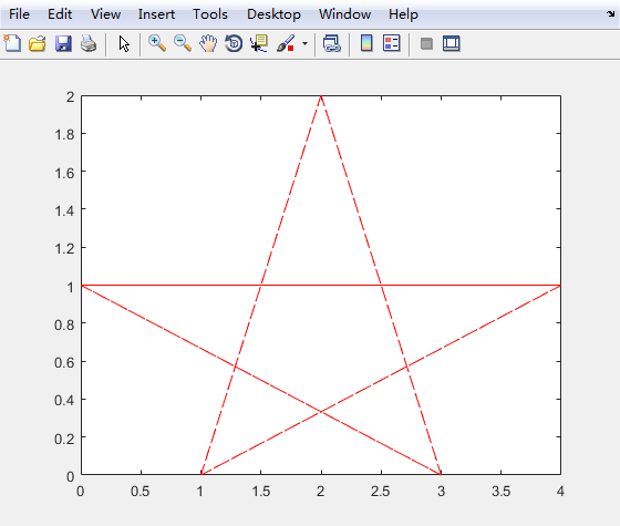
gplot

clc,clear,close all
a=[0,0,0,1,1;
    0,0,1,0,1;
    0,1,0,1,0;
    1,0,1,0,0;
    1,1,0,0,0;];
xy=[2 2;0 1;4 1;1 0;3 0];
gplot(a,xy,'r--')

图形标记

函数	说明
title	标题
xlabel/ylabel	坐标轴名称
legend	图例
xlim/ylim	xy坐标轴限度

三维图形

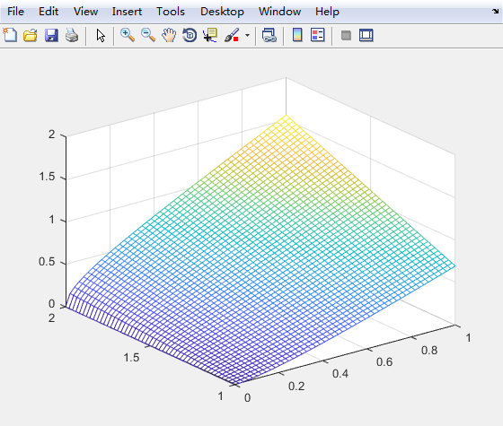
网格图

生成x，y方向向量

x=x1 : dx : xn;
y=y1 : dy : yn;

生成格点

[X,Y]=meshgrid(x,y);

绘制网格图

Z=f(x , y);
mesh(X,Y,Z);

clc,clear,close all
x=linspace(0,1,50);
y=linspace(1,2,50);
[X,Y]=meshgrid(x,y);
Z=zeros(50);
for m=1:50
    for n=1:50
        Z(m,n)=sqrt(X(m,n)*Y(m,n))*log(X(m,n)+Y(m,n));
    end
end
mesh(X,Y,Z);

其他函数

函数	说明
plot3	三维曲线
surf	曲面
contour	等值线图

动画

两种方式

帧数式

clc,clear,close all
x=-8:0.5:8;
[XX,YY]=meshgrid(x);
r=sqrt(XX.^2+YY.^2)+eps;
Z=sin(r)./r;
surf(Z);
theAxes=axis;
fmat=moviein(20);
for j=1:20
    surf(sin(2*pi*j/20)*Z,Z)
    axis(theAxes)
    fmat(:,j)=getframe;
end
movie(fmat,10)

句柄式

clc,clear,close all
animinit('onecart Animation')
%{Initializes a figure for Simulink animations.%}
axis([-2 6 -10 10]);
%{change the axis limits x [-2,6] y,[-10,10]%}
hold on;
u=2;
xy=[0 0 0 0 u u u+1 u+1 u u;
-1.2 0 1.2 0 0 1.2 1.2 -1.2 -1.2 0];
x=xy(1,:);
y=xy(2,:);
plot([-10 20],[-1.4 -1.4],'b-','LineWidth',2);
hndl=plot(x,y,'b-','EraseMode','XOR','LineWidth',2);
%{
Draw and erase the object by performing an exclusive OR (XOR) with the 
color of the screen beneath it. 
This mode does not damage the color of the objects beneath it. 
However, the object color depends on the color of whatever is beneath it 
on the display.
%}
set(gca,'UserData',hndl);
%{gca=Current Axes or chart,set it to the properties of hndl%}
t=1:0.025:100;
n=length(t);
for idx=1:n
u=2+exp(-0.01*t(idx))*cos(t(idx));
x=[0 0 0 0 u u u+1 u+1 u u];
hndl=get(gca,'UserData');
set(hndl,'XData',x);
%{set hndl's XData to x%}
title(['string,  t = ' num2str(t(idx),'%8.5e') ]);
%{set the title,remember to output number through this way%}
drawnow
frame=getframe(2);
%{get frame from figure 2%}
im{idx}=frame2im(frame);
end
filename = 'animating_by_handle.gif';
for idx=1:n
[A,map]=rgb2ind(im{idx},256);
%{RBG-->indexed image for gif onle support less than 256 bit%}
if idx ==1 
imwrite(A,map,filename,'gif','LoopCount',Inf,'DelayTime',0.01);
%{
LoopCount==Number of times to repeat the animation.
if you specify 0, the animation plays once.
If you specify the value 1, the animation plays twice, and so on.
ALoopCount value of Inf causes the animation to continuously loop.
%}
else
imwrite(A,map,filename,'gif','WriteMode','append','DelayTime',0.01);
%{
Writing mode, specified as the comma-separated pair 
consisting of'WriteMode'and either'overwrite'or'append'. 
In overwrite mode,imwrite overwrites an existing file,filename. 
In append mode, imwrite adds a single frame to the existing file.
%}
end
end

MATLAB编程

循环语句

for循环
while循环
区别：for循环用于已知循环次数，while循环用于不知道循环次数，只知道循环结束条件
break——结束当前层次循环
congtinue——当前循环不再往下进行

判断语句

if--elseif--else
switch--case--otherwise

终止控制语句

return——终止所有包含其的循环

插值拟合

插值——在离散数据的基础上补插连续函数，使得这条连续曲线通过全部给定的离散数据点。
拟合——构造一个函数，使该函数与原函数的差值在某种标准下最小
区别——已知点列，拟合是从整体上靠近，不需要经过点列；插值是完全经过点列

插值

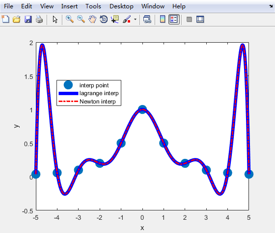
插值具有唯一性，所有插值方法的结果等价

拉格朗日插值

函数的matlab实现

function y=my_lagrange(x0,y0,x)
%come from Joe_zhouman,thanks for watching QAQ
m=length(x0);
n=length(x);
y=ones(1,n);
for tempi=1:n
    z=x(tempi);
    s=0;
    for tempj=1:m
        p=1;
        for tempk=1:m
            if tempk~=tempj
                p=p*(z-x0(tempk))/(x0(tempj)-x0(tempk));
            end
        end
        s=s+p*y0(tempj);
    end
    y(tempi)=s;
end
end

牛顿均差插值

函数的matlab实现

function y=my_newton_interp(x0,y0,x)
%come from Joe_zhouman,thanks for watching QAQ
m=length(x0);
n=length(x);
y=zeros(1,n);
df=y0;
for tempi=1:m-1
        for tempj=m:-1:tempi+1
            df(tempj)=(df(tempj)-df(tempj-1))/(x0(tempj)-x0(tempj-tempi));
        end
end
for tempk=1:n
    z=x(tempk);
    s=y0(1);
    p=z*ones(1,m)-x0;
    t=1;
    for tempi=1:m-1
        t=t*p(tempi);
        s=s+t*df(tempi+1);
    end
    y(tempk)=s;
end

插值的唯一性验证

clc,clear,close all
x=-5:5;
y=1./(1+x.^2);
x1=-5:0.01:5;
plot(x,y,'o','linewidth',8);
hold on
y1=my_lagrange(x,y,x1);
plot(x1,y1,'b','linewidth',5);
y2=my_newton_interp(x,y,x1);
plot(x1,y2,'r-.','linewidth',2);
xlabel('x');
ylabel('y');
legend('interp point','lagrange interp','Newton interp','location','best');

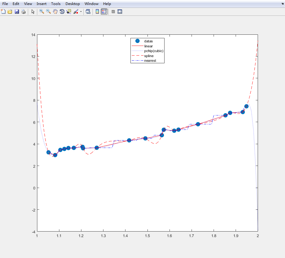
MATLAB插值函数

interp1

y=interp1(x0,y0,x,'method')

method	说明
linear	分段线性插值
cubic	分段三次多项式插值(在17a以上版本建议使用'pchip')
spline	分段三次样条插值（同cubic比还要求节点处光滑）
nearest	最邻近区域插值

clc,clear,close all
xdata=1+rand(1,20);
xdata=sort(xdata);
ydata=exp(xdata)+0.5*rand(1,20);
x=1:0.01:2;
y1=interp1(xdata,ydata,x,'linear');
y2=interp1(xdata,ydata,x,'pchip');
y3=interp1(xdata,ydata,x,'spline');
y4=interp1(xdata,ydata,x,'nearest');
plot(xdata,ydata,'o','linewidth',5);
hold on
plot(x,y1,'r',x,y2,'b:',x,y3,'r--',x,y4,'b-.')
legend('datas','linear','pchip(cubic)','spline','nearest','location','best')

拟合

多项式最小二乘拟合

推导

已知数据点 $$(x_1, y_1) (x_2, y_2) (x_3, y_3) ... (x_n,y_n) $$
其最小二乘解为函数 $$ y^* = a + bx $$
其方差

$$ \sigma^2=\sum (y^*_i-y_i ) ^ 2=\sum(a+bx_i-y_i)^2 $$

方差最小，则

$$ \frac{\partial{\sigma^2}}{\partial a}=\sum 2( a+bx_i-y_i ) = 0 $$
$$ \frac{\partial{\sigma^2}}{\partial b}=\sum 2( a+bx_i-y_i )x_i = 0 $$

整理得：

$$ na+\sum x_ib=\sum y_i $$

$$ \sum x_ia+\sum x_i^2b=\sum x_iy_i $$

写成矩阵形式

$$ \begin{pmatrix} n & \sum x_i \\ \sum x_i & \sum x_i^2 \end{pmatrix} * \begin{pmatrix} a \\ b \end{pmatrix} = \begin{pmatrix} \sum y_i \\ \sum x_iy_i \end{pmatrix} $$

解得

$$ a=\frac{\sum x_i^2(\sum y_i)-(\sum x_iy_i)(\sum x_i)}{n\sum x_i^2 - (\sum x_i)^2} $$ $$ b=\frac{n\sum x_iy_i-(\sum x_i)(\sum y_i)}{n\sum x_i^2 - (\sum x_i)^2} $$

matlab实现

function [a,b]=my_linear_fitting(x,y)
S=[length(x),sum(x);
    sum(x),sum(x.^2)];
r=[sum(y);sum(x.*y)];
T=S\r;
a=T(1,:);
b=T(2,:);
end

matlab自带函数
polyfit

P=polyfit(X,Y,N)

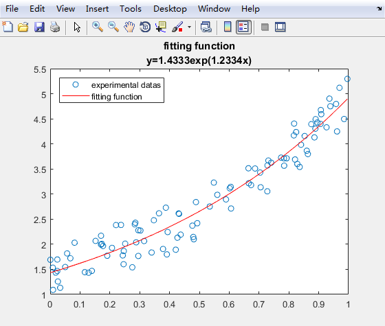
非线性最小二乘拟合

lsqcurvefit

clc,clear,close all
xdata=rand(1,100);
xdata=sort(xdata);
ydata=exp(1.5.*xdata)+rand(1,100);
fun=@(t,xdata)t(1)*exp(t(2)*xdata);
startpoint=[0,10];
t=lsqcurvefit(fun,startpoint,xdata,ydata);
ydata0=fun(t,xdata);
plot(xdata,ydata,'o',xdata,ydata0,'r-')
title({'fitting function';['y=',num2str(t(1)),'exp(',num2str(t(2)),'x)']})
legend('experimental datas','fitting function','Location','northwest')

lsqnonlin

clc,clear,close all
xdata=rand(1,100);
xdata=sort(xdata);
ydata=exp(1.5.*xdata)+rand(1,100);
fun=@(t)t(1)*exp(t(2)*xdata)-ydata;
startpoint=[0,10];
t=lsqnonlin(fun,startpoint);
ydata0=fun(t)+ydata;
plot(xdata,ydata,'o',xdata,ydata0,'r-')
title({'fitting function';['y=',num2str(t(1)),'exp(',num2str(t(2)),'x)']})
legend('experimental datas','fitting function','Location','northwest')

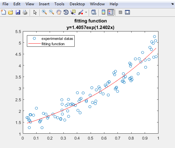
differences
算法不同,导致输入的function的要求不同

对于lsqcurvefit,其算法为

$$ min\sum [F(x,xdata)-ydata]^2 $$

对于lsqnonlin,其算法为

$$ min\sum F(x)^2 $$

输入的fun需满足算法需求.

微分方程求解

基本微积分运算

运算	函数	调用	说明
求极限	limit	limit(fun,x,x0)	fun为函数或符号函数
求导数	diff	diff(fun,n)	fun为函数或抽象函数
求积分	int	int(f,r,x0,x1)	fun为函数

数值积分

数值积分常用方法

方法	函数	调用
中点法
梯形法	trapz
Simpson法	quad	quad('fname',a,b,tol,trace)
Newton-Cotes法	quadl	quadl('fname',a,b,tol,trace)

常微分方程求解

最简单的形式,dsolve求符号解
dsolve('equation','condition','v')
- equation---所求方程
- condition---初值条件
- v---解的自变量
 
 注:
 a. 若无'v',则接触的函数以t为自变量
 b. y永远不能做自变量
 c. 除y及自变量v以外的变量被视作参数
数值解

欧拉法
- 向前欧拉法(显式)
- 向后欧拉法(隐式)
- 梯形公式
- 改进欧拉法
龙格库塔法
亚当斯方法
- 亚当斯外推公式
- 亚当斯内推公式
- 亚当斯矫正公式
- hamming法

自带函数
ode45
ode23
....

方程(组)求解

递推算法-方程求根

循环迭代法

将求y=f(x)的根转化为求y=ϕ(x) 与 y=x的交点
从初始点x0出发,沿x=x0走到y=ϕ(x),得到点(x0,ϕ(x0)),再沿y=ϕ(x0)走到y=x,得到(x1,ϕ(x1)),如此进行下去,不断逼近方程的解(x∗,y∗)

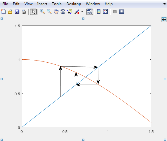
迭代的收敛性:
ϕ(x)在[a,b]满足
a<ϕ(x)
ϕ(x)=x+1
ϕ(x)=1+x1

function y=my_loop_iteration(fun,x0,tol)
y0=fun(x0);
while abs(fun(x0)-x0)>tol
    x0=y0;
    y0=fun(x0);
end
y=y0;
end

牛顿迭代法

function root=my_newton_iteration(fun,x0,tol1,tol2)
y=fun(x0);
if nargin<4
    tol2=1e-5;
end
if nargin==3
    tol1=1e-6;
end
dy=(fun(x0+tol2)-y)/tol2;
if dy==0
    error('dy/dx=0 at x0');
end
d=y/dy;
while abs(d)>tol1
    x0=x0-d;
    y=fun(x0);
    dy=(fun(x0+tol2)-y)/tol2;
    if dy==0
        error('dy/dx=0 at iteration');
    end
    d=y/dy;
end
root=x0;
end

二分法

线性方程组求解

Gauss消元法

追赶法

高斯-赛德尔迭代法

function x=my_gauss_seidel_iteration(A,b,x0,tol)
if nargin<4
    tol=1e-6;
end
n=size(A);
k=length(b);
if (n(1)~=n(2))||(n(1)~=k)
    error('check your input');
    return
end
D=diag(diag(A));
L=-tril(A)+D;
U=-triu(A)+D;
DL=D-L;
At=DL\U;
bt=DL\b;
x=At*x0+bt;
while norm(x-x0)>tol
    x=x0;
    x0=At*x+bt;
end
end

雅可比迭代法

概率统计

统计图

函数	说明	备注
boxplot	盒图
bar	条形图
histogram	直方图
pie	饼图

本文由 joe_zhouman 创作，采用知识共享署名4.0 国际许可协议进行许可
本站文章除注明转载/出处外，均为本站原创或翻译，转载前请务必署名
最后编辑时间为:2019-07-15 00:00:00

Matlab-基础应用